R&D Blog
Volatility Clustering: Part 2 | Data Analysis
I. Trading Strategy
Concept: Large price moves tend to be followed by large price moves, and small price moves tend to be followed by small price moves (Volatility Clustering). Research Question: Can we improve performance of the original volatility clustering model via standard deviation filtering of large price moves? Specification: Table 1. Results: Figure 1-4. Trade Setup: We identify large price moves via Volatility Breakout Pattern. Volatility Breakout Pattern is defined as the price true range exceeding N standard deviations. Trade Entry/Exit: Table 1. Portfolio: 42 futures markets from four major market sectors (commodities, currencies, interest rates, and equity indexes). Data: 39 years since 1980. Testing Platform: MATLAB®.
II. Sensitivity Test
All 3-D charts are followed by 2-D contour charts for Profit Factor, Sharpe Ratio, Ulcer Performance Index, Avg. Return, Maximum Drawdown, Percent Profitable Trades, and Avg. Win / Avg. Loss Ratio. The final picture shows sensitivity of Equity Curve.
Scenario #1: Large price moves in one direction are followed by large price moves in the opposite direction (i.e. volatility clustering with a price drift reversal). Tested Variables: MA_Length & Time_Index (Definitions: Table 1):
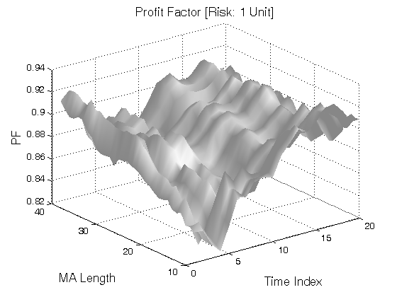
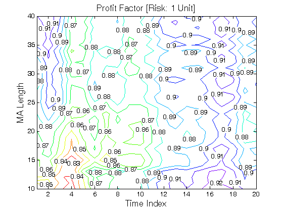
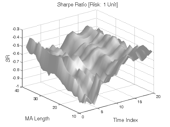
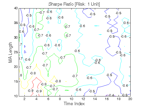
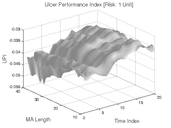
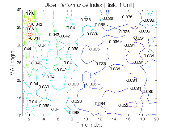
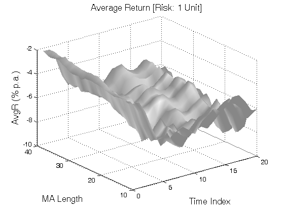
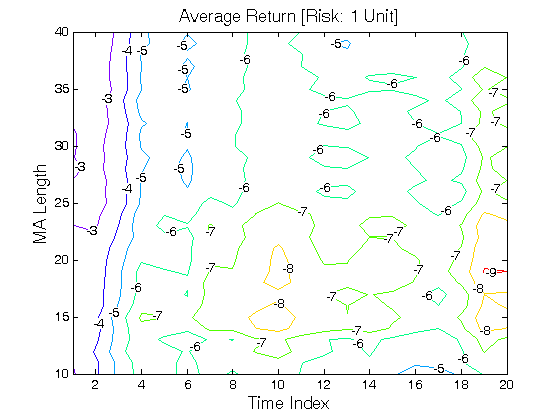
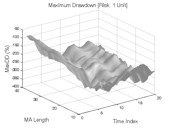
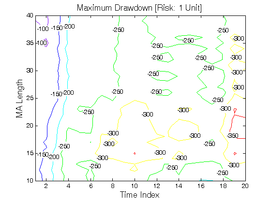
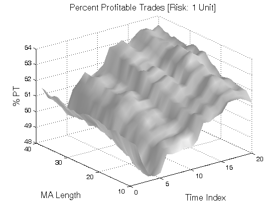
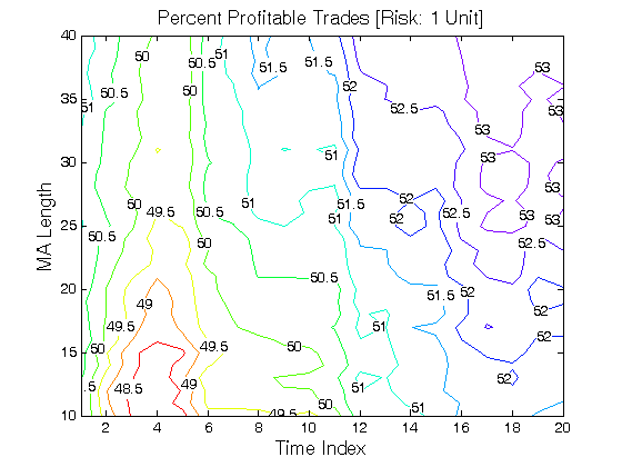
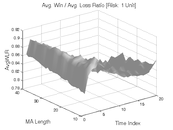
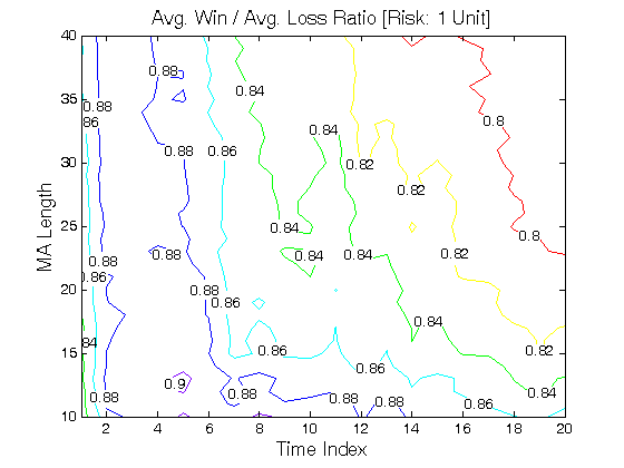
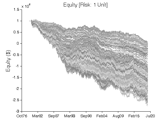
Figure 1 | Portfolio Performance for Scenario #1 (Inputs: Table 1; Commission & Slippage: $0).
Scenario #2: Large price moves in one direction are followed by large price moves in the same direction (i.e. volatility clustering with a price drift continuation). Tested Variables: MA_Length & Time_Index (Definitions: Table 1):

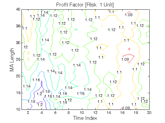
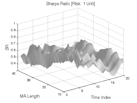
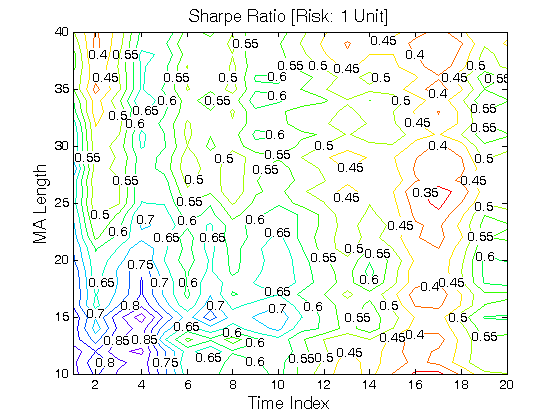


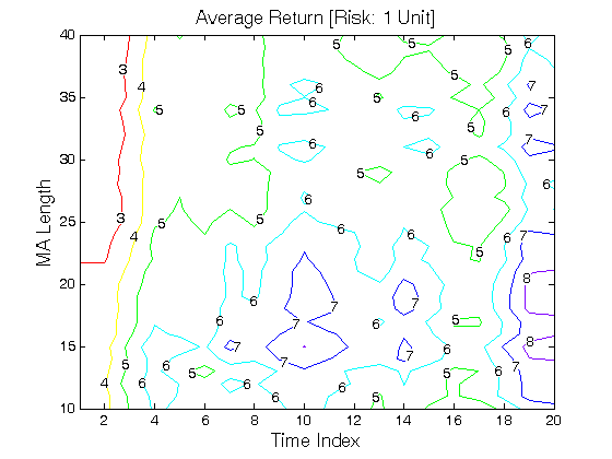
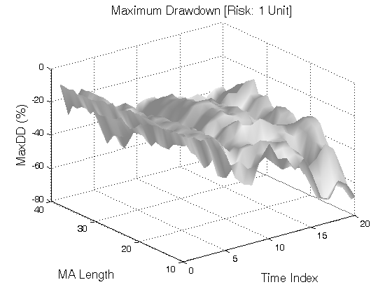
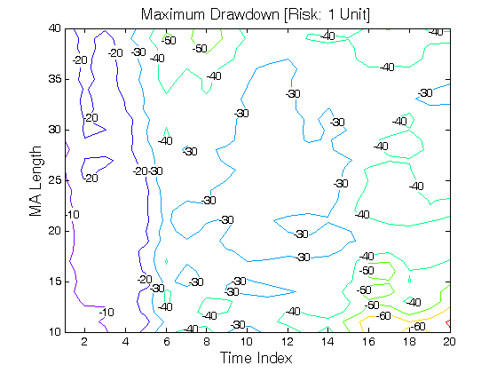

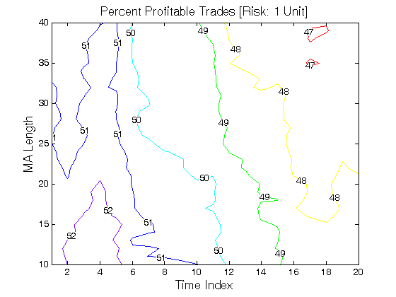
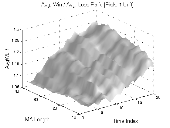


Figure 2 | Portfolio Performance for Scenario #2 (Inputs: Table 1; Commission & Slippage: $0).
| STRATEGY | SPECIFICATION | PARAMETERS |
| Auxiliary Variables: | Max_High[i] = max(High[i − X +1] : High[i]). Min_Low[i] = min(Low[i − X +1] : Low[i]). True_High[i] = max(Close[i − X], Max_High[i]). True_Low[i] = min(Close[i − X], Min_Low[i]). True_Range[i] = True_High[i] − True_Low[i]. Index: i ~ Current Bar. | X = 2; |
| Setup: | Volatility Breakout Pattern is defined as the X-day True_Range exceeding N standard deviations: True_Range[i] > Average(True_Range[i] over a period of MA_Length) + N * StDev(True_Range[i] over a period of MA_Length). Index: i ~ Current Bar. | X = 2; N = 2; MA_Length = [10, 40], Step = 1; |
| Filter: | Scenario #1: Price Reversal Long Trades: On the Setup bar, Open[i − X +1] > Close[i]. Short Trades: On the Setup bar, Open[i − X +1] < Close[i]. Index: i ~ Current Bar. Scenario #2: Price Continuation Long Trades: On the Setup bar, Open[i − X +1] < Close[i]. Short Trades: On the Setup bar, Open[i − X +1] > Close[i]. Index: i ~ Current Bar. | X=2; |
| Entry: | Buy/sell orders at the open. | |
| Exit: | Time Exit: nth day at the close, n = Time_Index. Stop Loss Exit: ATR(ATR_Length) is the Average True Range over a period of ATR_Length. ATR_Stop is a multiple of ATR(ATR_Length). Long Trades: A sell stop is placed at [Entry − ATR(ATR_Length) * ATR_Stop]. Short Trades: A buy stop is placed at [Entry + ATR(ATR_Length) * ATR_Stop]. | Time_Index = [1, 20], Step = 1; ATR_Length = 20; ATR_Stop = 6; |
| Sensitivity Test: | MA_Length = [10, 40], Step = 1 Time_Index = [1, 20], Step = 1 | |
| Position Sizing: | Initial_Capital = $1,000,000 Constant_$_Risk = $10,000 per Trade (Vol. Adjusted) Portfolio = 42 US Futures ATR_Stop = 6 (ATR ~ Average True Range) ATR_Length = 20 | |
| Data: | 42 futures markets; 39 years (1980/01/01−2019/07/31) |
Table 1 | Specification: Trading Strategy.
III. Benchmarking
Scenario #1: Large price moves in one direction are followed by large price moves in the opposite direction (i.e. volatility clustering with a price drift reversal). Scenario #2: Large price moves in one direction are followed by large price moves in the same direction (i.e. volatility clustering with a price drift continuation).
We benchmark Scenario #1 (Table 2) against Scenario #2 (Table 3):
Case #A: X = 2; MA_Length = 20; Time_Index = 1.
Case #B: X = 2; MA_Length = 20; Time_Index = 2.
Case #C: X = 2; MA_Length = 20; Time_Index = 3.
Case #D: X = 2; MA_Length = 20; Time_Index = 4.
| Scenario #1 | Case #A | Case #B | Case #C | Case #D |
| Net Profit ($) | (1,316,906) | (1,400,986) | (1,932,822) | (2,429,407) |
| Sharpe Ratio | (0.78) | (0.64) | (0.73) | (0.81) |
| Ulcer Performance Index (UPI) | (0.04) | (0.04) | (0.04) | (0.04) |
| Profit Factor | 0.87 | 0.88 | 0.86 | 0.85 |
| Avg. Return (%) | (3.21) | (3.42) | (4.72) | (5.93) |
| Max. Drawdown (%) | (136.70) | (145.18) | (196.90) | (243.53) |
| Percent Profitable Trades (%) | 50.83 | 49.98 | 49.32 | 48.85 |
| Avg. Win / Avg. Loss Ratio | 0.84 | 0.88 | 0.89 | 0.89 |
Table 2 | Inputs: Table 1; Constant_$_Risk: $10,000 per Trade (Vol. Adjusted); Commission & Slippage: $0 Round Turn.
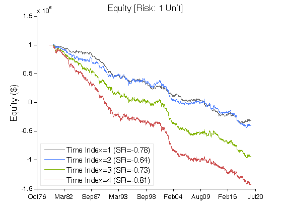
Figure 3 | Equity Curves for Scenario #1 (Table 2).
| Scenario #2 | Case #A | Case #B | Case #C | Case #D |
| Net Profit ($) | 1,274,693 | 1,356,156 | 1,850,865 | 2,288,624 |
| Sharpe Ratio | 0.76 | 0.61 | 0.69 | 0.75 |
| Ulcer Performance Index (UPI) | 1.20 | 0.77 | 1.22 | 1.38 |
| Profit Factor | 1.14 | 1.13 | 1.15 | 1.17 |
| Avg. Return (%) | 3.11 | 3.31 | 4.52 | 5.59 |
| Max. Drawdown (%) | (7.39) | (13.04) | (12.15) | (13.96) |
| Percent Profitable Trades (%) | 51.23 | 51.07 | 51.74 | 52.06 |
| Avg. Win / Avg. Loss Ratio | 1.09 | 1.09 | 1.08 | 1.08 |
Table 3 | Inputs: Table 1; Constant_$_Risk: $10,000 per Trade (Vol. Adjusted); Commission & Slippage: $0 Round Turn.
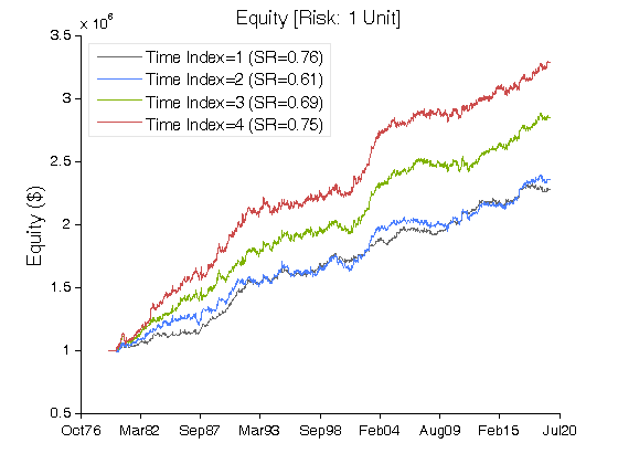
Figure 4 | Equity Curves for Scenario #2 (Table 3).
IV. Basic Concepts
B. Mandelbrot, The (mis)Behavior of Markets:
Concentration is common. Look at a map of gold deposits around the world: You see clusters of gold veins – in South Africa and Zimbabwe, in the far reaches of Siberia and elsewhere. This is not total chance; millennia of real tectonic forces gradually worked it that way. Understanding concentration is crucial to many businesses, especially insurance. A recent study of tornado damage in Texas, Louisiana, and Mississippi found 90 percent of the claims came from just 5 percent of the insured land area.
V. Summary
On a large portfolio of futures markets, Scenario #2 (Table 3) outperforms Scenario #1 (Table 2). Research Question: Can we improve performance of the original volatility clustering model via standard deviation filtering of large price moves? Not in a significant way.
Related Entries: Volatility Clustering: Part 1 | Volatility Clustering: Part 3 | Narrow Range N-Day Pattern
Related Topics: (Public) Trading Strategies
CFTC RULE 4.41: HYPOTHETICAL OR SIMULATED PERFORMANCE RESULTS HAVE CERTAIN LIMITATIONS. UNLIKE AN ACTUAL PERFORMANCE RECORD, SIMULATED RESULTS DO NOT REPRESENT ACTUAL TRADING. ALSO, SINCE THE TRADES HAVE NOT BEEN EXECUTED, THE RESULTS MAY HAVE UNDER-OR-OVER COMPENSATED FOR THE IMPACT, IF ANY, OF CERTAIN MARKET FACTORS, SUCH AS LACK OF LIQUIDITY. SIMULATED TRADING PROGRAMS IN GENERAL ARE ALSO SUBJECT TO THE FACT THAT THEY ARE DESIGNED WITH THE BENEFIT OF HINDSIGHT. NO REPRESENTATION IS BEING MADE THAT ANY ACCOUNT WILL OR IS LIKELY TO ACHIEVE PROFIT OR LOSSES SIMILAR TO THOSE SHOWN.
RISK DISCLOSURE: U.S. GOVERNMENT REQUIRED DISCLAIMER | CFTC RULE 4.41
Codes: matlab/data/volatility-clustering-2