R&D Blog
Volatility Clustering: Part 1 | Data Analysis
I. Trading Strategy
Concept: Large price moves tend to be followed by large price moves, and small price moves tend to be followed by small price moves (Volatility Clustering). Research Question: Is there a tendency of large price moves in one direction to be followed by large price moves in the opposite direction? Specification: Table 1. Results: Figure 1-4. Trade Setup: We identify large price moves via Wide Range X-Day pattern. Wide Range X-Day pattern is defined as the widest range from true high to true low of any X-day period relative to any X-day period within the previous Y market days. Trade Entry/Exit: Table 1. Portfolio: 42 futures markets from four major market sectors (commodities, currencies, interest rates, and equity indexes). Data: 39 years since 1980. Testing Platform: MATLAB®.
II. Sensitivity Test
All 3-D charts are followed by 2-D contour charts for Profit Factor, Sharpe Ratio, Ulcer Performance Index, Avg. Return, Maximum Drawdown, Percent Profitable Trades, and Avg. Win / Avg. Loss Ratio. The final picture shows sensitivity of Equity Curve.
Scenario #1: Large price moves in one direction are followed by large price moves in the opposite direction (i.e. volatility clustering with a price drift reversal). Tested Variables: Y & Time_Index (Definitions: Table 1):
Figure 1 | Portfolio Performance for Scenario #1 (Inputs: Table 1; Commission & Slippage: $0).
Scenario #2: Large price moves in one direction are followed by large price moves in the same direction (i.e. volatility clustering with a price drift continuation). Tested Variables: Y & Time_Index (Definitions: Table 1):
Figure 2 | Portfolio Performance for Scenario #2 (Inputs: Table 1; Commission & Slippage: $0).
| STRATEGY | SPECIFICATION | PARAMETERS |
| Auxiliary Variables: | Max_High[i] = max(High[i − X +1] : High[i]). Min_Low[i] = min(Low[i − X +1] : Low[i]). True_High[i] = max(Close[i − X], Max_High[i]). True_Low[i] = min(Close[i − X], Min_Low[i]). Index: i ~ Current Bar. | X = 2; |
| Setup: | Wide Range X-Day pattern is defined as the widest range from True_High to True_Low of any X-day period relative to any X-day period within the previous Y market days. In the sensitivity test, we research the size of the look back period Y. | X = 2; Y = [10, 40], Step = 1; |
| Filter: | Scenario #1: Price Reversal Long Trades: On the Setup bar, Open[i − X +1] > Close[i]. Short Trades: On the Setup bar, Open[i − X +1] < Close[i]. Index: i ~ Current Bar. Scenario #2: Price Continuation Long Trades: On the Setup bar, Open[i − X +1] < Close[i]. Short Trades: On the Setup bar, Open[i − X +1] > Close[i]. Index: i ~ Current Bar. | X=2; |
| Entry: | Buy/sell orders at the open. | |
| Exit: | Time Exit: nth day at the close, n = Time_Index. Stop Loss Exit: ATR(ATR_Length) is the Average True Range over a period of ATR_Length. ATR_Stop is a multiple of ATR(ATR_Length). Long Trades: A sell stop is placed at [Entry − ATR(ATR_Length) * ATR_Stop]. Short Trades: A buy stop is placed at [Entry + ATR(ATR_Length) * ATR_Stop]. | Time_Index = [1, 20], Step = 1; ATR_Length = 20; ATR_Stop = 6; |
| Sensitivity Test: | Y = [10, 40], Step = 1 Time_Index = [1, 20], Step = 1 | |
| Position Sizing: | Initial_Capital = $1,000,000 Constant_$_Risk = $10,000 per Trade (Vol. Adjusted) Portfolio = 42 US Futures ATR_Stop = 6 (ATR ~ Average True Range) ATR_Length = 20 | |
| Data: | 42 futures markets; 39 years (1980/01/01−2019/07/31) |
Table 1 | Specification: Trading Strategy.
III. Benchmarking
Scenario #1: Large price moves in one direction are followed by large price moves in the opposite direction (i.e. volatility clustering with a price drift reversal). Scenario #2: Large price moves in one direction are followed by large price moves in the same direction (i.e. volatility clustering with a price drift continuation).
We benchmark Scenario #1 (Table 2) against Scenario #2 (Table 3):
Case #A: X = 2; Y = 20; Time_Index = 1.
Case #B: X = 2; Y = 20; Time_Index = 2.
Case #C: X = 2; Y = 20; Time_Index = 3.
Case #D: X = 2; Y = 20; Time_Index = 4.
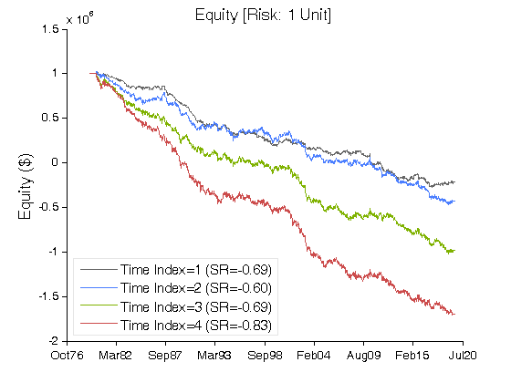
| Scenario #1 | Case #A | Case #B | Case #C | Case #D |
| Net Profit ($) | (1,216,982) | (1,432,035) | (1,983,709) | (2,698,844) |
| Sharpe Ratio | (0.69) | (0.60) | (0.69) | (0.83) |
| Ulcer Performance Index (UPI) | (0.04) | (0.04) | (0.04) | (0.04) |
| Profit Factor | 0.89 | 0.90 | 0.88 | 0.86 |
| Avg. Return (%) | (2.97) | (3.49) | (4.84) | (6.59) |
| Max. Drawdown (%) | (128.71) | (149.33) | (202.36) | (271.11) |
| Percent Profitable Trades (%) | 51.26 | 50.19 | 49.41 | 48.94 |
| Avg. Win / Avg. Loss Ratio | 0.85 | 0.89 | 0.90 | 0.90 |
Table 2 | Inputs: Table 1; Constant_$_Risk: $10,000 per Trade (Vol. Adjusted); Commission & Slippage: $0 Round Turn.

Figure 3 | Equity Curves for Scenario #1 (Table 2).
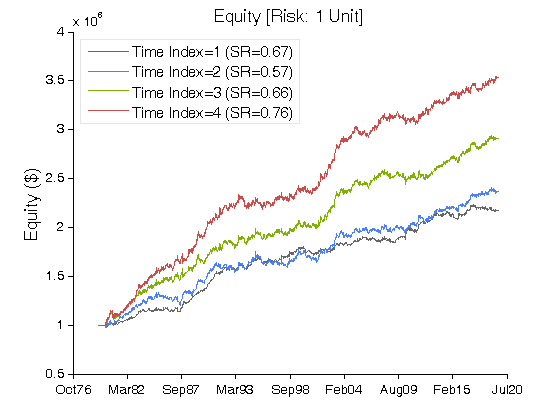
| Scenario #2 | Case #A | Case #B | Case #C | Case #D |
| Net Profit ($) | 1,174,853 | 1,363,818 | 1,908,321 | 2,530,514 |
| Sharpe Ratio | 0.67 | 0.57 | 0.66 | 0.76 |
| Ulcer Performance Index (UPI) | 0.97 | 0.67 | 1.13 | 1.29 |
| Profit Factor | 1.11 | 1.11 | 1.13 | 1.15 |
| Avg. Return (%) | 2.87 | 3.33 | 4.66 | 6.18 |
| Max. Drawdown (%) | (8.80) | (16.24) | (14.61) | (15.28) |
| Percent Profitable Trades (%) | 50.77 | 50.95 | 51.63 | 51.95 |
| Avg. Win / Avg. Loss Ratio | 1.08 | 1.07 | 1.06 | 1.07 |
Table 3 | Inputs: Table 1; Constant_$_Risk: $10,000 per Trade (Vol. Adjusted); Commission & Slippage: $0 Round Turn.

Figure 4 | Equity Curves for Scenario #2 (Table 3).
IV. Basic Concepts
B. Mandelbrot, The (mis)Behavior of Markets:
The size of the price changes clearly cluster together. Big changes often come together in rapid succession, like a fusillade of cannon fire; then come long stretches of minor changes, like the pop of toy guns. There is scaling here, too: If you zoom in on an individual cluster of big changes, you find it is made up of smaller clusters. Zoom again, and you find even finer clusters. It is a fractal structure. Nor is it just the price changes of interest; at times, the price levels also exhibit some kind of irregular regularity. The charts sometimes rise or fall in long waves, or with small waves superimposed on bigger waves. But none of these phenomena – clusters of volatility, or irregular trends – resemble any of the cycles, waves, or other patterns that characterize those aspects of nature controlled through well-established science. There are no familiar sine or cosine waves, with regular periods, of the kind that undulate evenly across the green screen of an old oscilloscope. These peculiar patterns cannot be predicted; and so humans who bet on them often lose. Yet there clearly is a system to them. It is as if the charts have a memory of their past. If the price changes start to cluster, or the prices themselves start to rise, they have a slight tendency to keep doing so for a while – and then, without warning, they stop. They may even flip to the opposite trend.
V. Summary
On a large portfolio of futures markets, Scenario #2 (Table 3) outperforms Scenario #1 (Table 2).
Related Entries: Volatility Clustering: Part 2 | Volatility Clustering: Part 3 | Narrow Range N-Day Pattern
Related Topics: (Public) Trading Strategies
CFTC RULE 4.41: HYPOTHETICAL OR SIMULATED PERFORMANCE RESULTS HAVE CERTAIN LIMITATIONS. UNLIKE AN ACTUAL PERFORMANCE RECORD, SIMULATED RESULTS DO NOT REPRESENT ACTUAL TRADING. ALSO, SINCE THE TRADES HAVE NOT BEEN EXECUTED, THE RESULTS MAY HAVE UNDER-OR-OVER COMPENSATED FOR THE IMPACT, IF ANY, OF CERTAIN MARKET FACTORS, SUCH AS LACK OF LIQUIDITY. SIMULATED TRADING PROGRAMS IN GENERAL ARE ALSO SUBJECT TO THE FACT THAT THEY ARE DESIGNED WITH THE BENEFIT OF HINDSIGHT. NO REPRESENTATION IS BEING MADE THAT ANY ACCOUNT WILL OR IS LIKELY TO ACHIEVE PROFIT OR LOSSES SIMILAR TO THOSE SHOWN.
RISK DISCLOSURE: U.S. GOVERNMENT REQUIRED DISCLAIMER | CFTC RULE 4.41
Codes: matlab/data/volatility-clustering-1


