R&D Blog
Volatility Clustering: Part 3 | Data Analysis
I. Trading Strategy
Concept: Opening Range Breakout (ORB) with Volatility Clustering (Large price moves tend to be followed by large price moves, and small price moves tend to be followed by small price moves). Research Question: Can we improve performance of the original volatility clustering model via Opening Range Breakout (ORB)? Specification: Table 1. Results: Figure 1-4. Trade Setup: We identify large price moves via Wide Range X-Day pattern. Wide Range X-Day pattern is defined as the widest range from true high to true low of any X-day period relative to any X-day period within the previous Y market days. Trade Entry/Exit: Table 1. Portfolio: 42 futures markets from four major market sectors (commodities, currencies, interest rates, and equity indexes). Data: 39 years since 1980. Testing Platform: MATLAB®.
II. Sensitivity Test
All 3-D charts are followed by 2-D contour charts for Profit Factor, Sharpe Ratio, Ulcer Performance Index, Avg. Return, Maximum Drawdown, Percent Profitable Trades, and Avg. Win / Avg. Loss Ratio. The final picture shows sensitivity of Equity Curve.
Scenario #1: Large price moves in one direction are followed by large price moves in the opposite direction (i.e. volatility clustering with a price drift reversal). Tested Variables: Y & Time_Index (Definitions: Table 1):
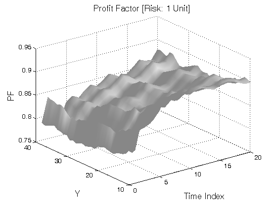
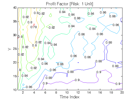
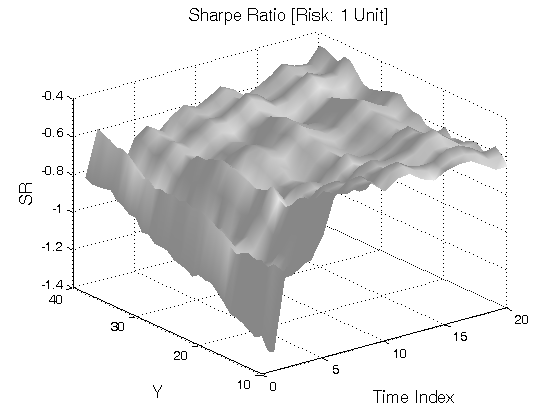
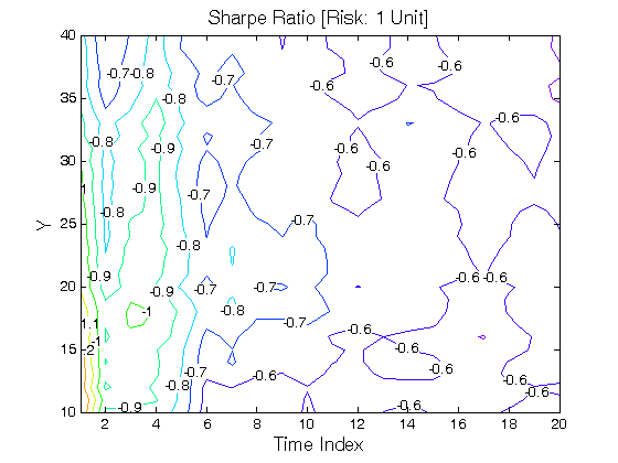
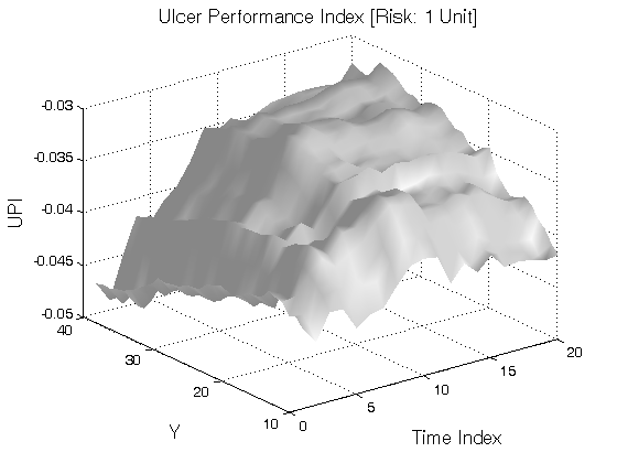
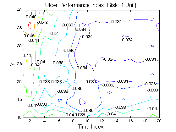
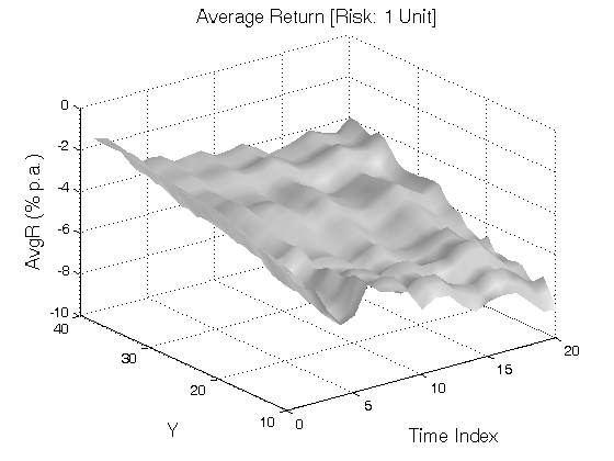
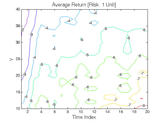

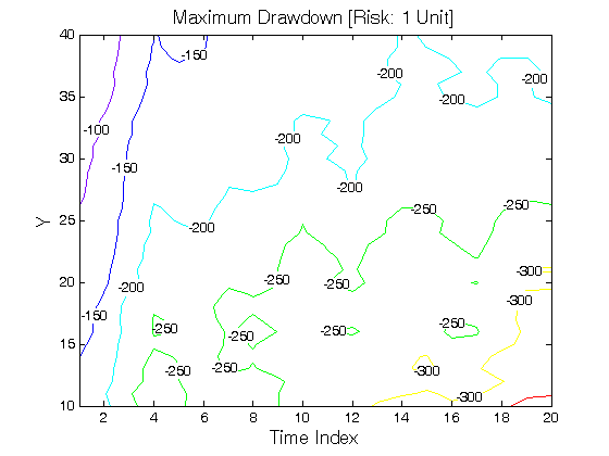
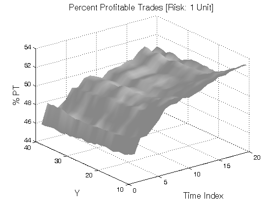
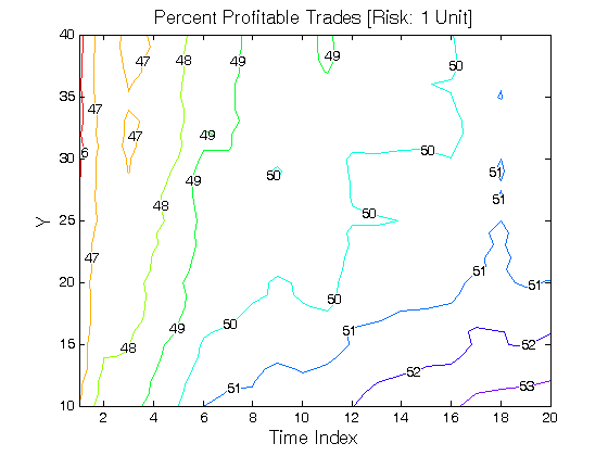
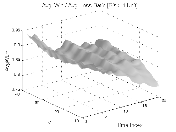
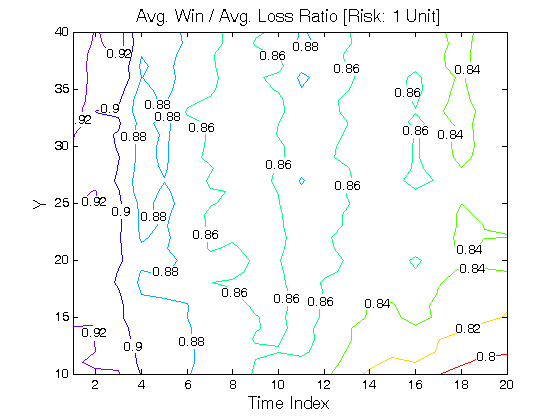
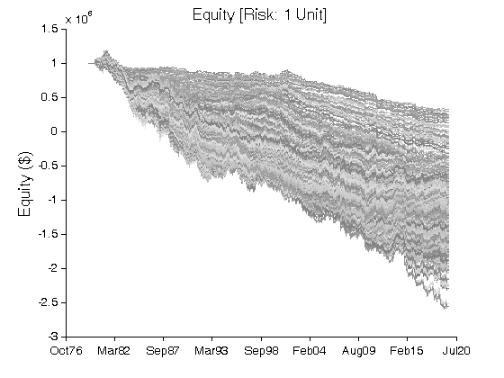
Figure 1 | Portfolio Performance for Scenario #1 (Inputs: Table 1; Commission & Slippage: $0).
Scenario #2: Large price moves in one direction are followed by large price moves in the same direction (i.e. volatility clustering with a price drift continuation). Tested Variables: Y & Time_Index (Definitions: Table 1):
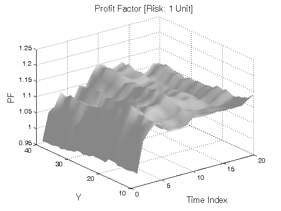

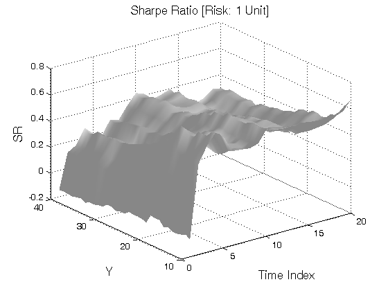
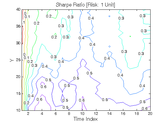
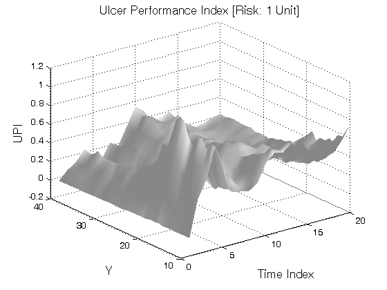
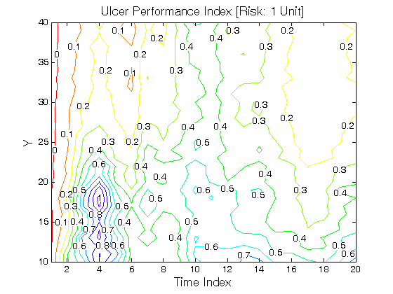
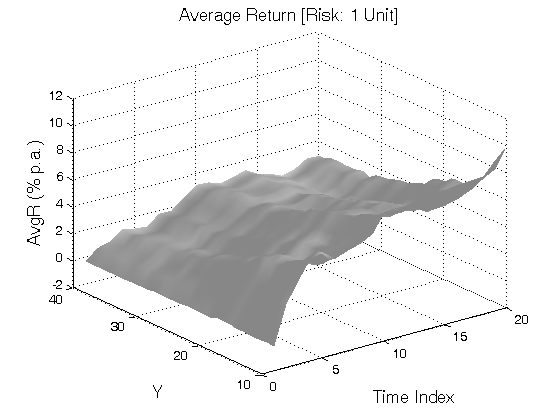
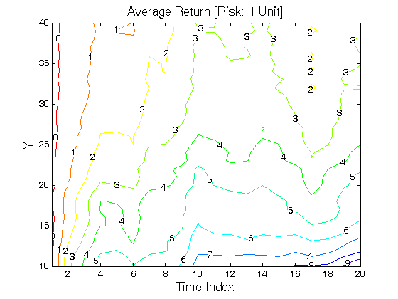

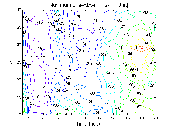
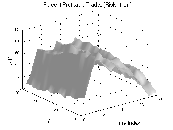
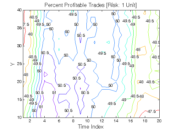
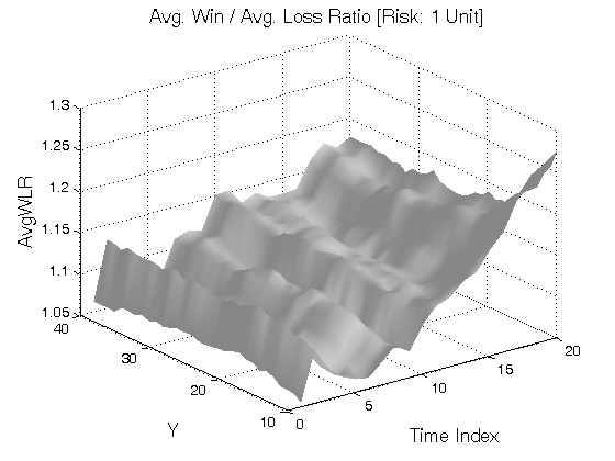
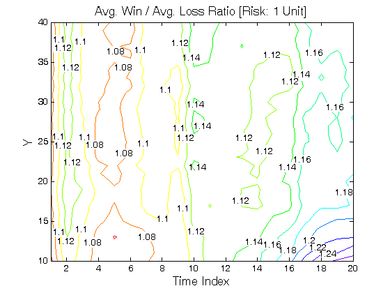

Figure 2 | Portfolio Performance for Scenario #2 (Inputs: Table 1; Commission & Slippage: $0).
| STRATEGY | SPECIFICATION | PARAMETERS |
| Auxiliary Variables: | Max_High[i] = max(High[i − X +1] : High[i]). Min_Low[i] = min(Low[i − X +1] : Low[i]). True_High[i] = max(Close[i − X], Max_High[i]). True_Low[i] = min(Close[i − X], Min_Low[i]). Index: i ~ Current Bar. | X = 2; |
| Setup: | Wide Range X-Day pattern is defined as the widest range from True_High to True_Low of any X-day period relative to any X-day period within the previous Y market days. In the sensitivity test, we research the size of the look back period Y. | X = 2; Y = [10, 40], Step = 1; |
| Filter: | Scenario #1: Price Reversal Long Trades: On the Setup bar, Open[i − X +1] > Close[i]. Short Trades: On the Setup bar, Open[i − X +1] < Close[i]. Index: i ~ Current Bar. Scenario #2: Price Continuation Long Trades: On the Setup bar, Open[i − X +1] < Close[i]. Short Trades: On the Setup bar, Open[i − X +1] > Close[i]. Index: i ~ Current Bar. | X=2; |
| Entry: | Noise: The difference between the open for each day and the closest extreme to the open on each day (Noise[i] = min(High[i] − Open[i], Open[i] − Low[i])). Index: i ~ Current Bar. Average Noise: The simple moving average of Noise over a period of Stretch_Length. Stretch: Stretch[i] = Average_Noise[i] * Stretch_Multiple. Index: i ~ Current Bar. Opening Range Breakout (ORB): A trade is taken at a predetermined amount above/below the open. The predetermined amount is the Stretch (defined above). Long Trades: A buy stop is placed at [Open + Stretch]. Short Trades: A sell stop is placed at [Open − Stretch]. | Stretch_Length = 10; Stretch_Multiple = 2; |
| Exit: | Time Exit: nth day at the close, n = Time_Index. Stop Loss Exit: ATR(ATR_Length) is the Average True Range over a period of ATR_Length. ATR_Stop is a multiple of ATR(ATR_Length). Long Trades: A sell stop is placed at [Entry − ATR(ATR_Length) * ATR_Stop]. Short Trades: A buy stop is placed at [Entry + ATR(ATR_Length) * ATR_Stop]. | Time_Index = [1, 20], Step = 1; ATR_Length = 20; ATR_Stop = 6; |
| Sensitivity Test: | Y = [10, 40], Step = 1 Time_Index = [1, 20], Step = 1 | |
| Position Sizing: | Initial_Capital = $1,000,000 Constant_$_Risk = $10,000 per Trade (Vol. Adjusted) Portfolio = 42 US Futures ATR_Stop = 6 (ATR ~ Average True Range) ATR_Length = 20 | |
| Data: | 42 futures markets; 39 years (1980/01/01−2019/07/31) |
Table 1 | Specification: Trading Strategy.
III. Benchmarking
Scenario #1: Large price moves in one direction are followed by large price moves in the opposite direction (i.e. volatility clustering with a price drift reversal). Scenario #2: Large price moves in one direction are followed by large price moves in the same direction (i.e. volatility clustering with a price drift continuation).
We benchmark Scenario #1 (Table 2) against Scenario #2 (Table 3):
Case #A: X = 2; Y = 20; Time_Index = 1.
Case #B: X = 2; Y = 20; Time_Index = 2.
Case #C: X = 2; Y = 20; Time_Index = 3.
Case #D: X = 2; Y = 20; Time_Index = 4.
| Scenario #1 | Case #A | Case #B | Case #C | Case #D |
| Net Profit ($) | (1,122,231) | (1,374,939) | (1,894,884) | (2,105,343) |
| Sharpe Ratio | (1.09) | (0.85) | (0.94) | (0.90) |
| Ulcer Performance Index (UPI) | (0.04) | (0.04) | (0.04) | (0.04) |
| Profit Factor | 0.80 | 0.84 | 0.82 | 0.83 |
| Avg. Return (%) | (2.74) | (3.36) | (4.62) | (5.14) |
| Max. Drawdown (%) | (112.96) | (140.92) | (191.12) | (213.29) |
| Percent Profitable Trades (%) | 46.41 | 47.79 | 47.57 | 48.29 |
| Avg. Win / Avg. Loss Ratio | 0.92 | 0.91 | 0.90 | 0.88 |
Table 2 | Inputs: Table 1; Constant_$_Risk: $10,000 per Trade (Vol. Adjusted); Commission & Slippage: $0 Round Turn.
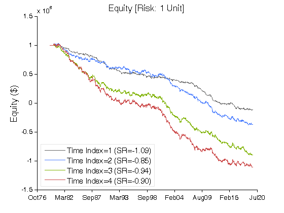
Figure 3 | Equity Curves for Scenario #1 (Table 2).
| Scenario #2 | Case #A | Case #B | Case #C | Case #D |
| Net Profit ($) | (106,701) | 425,660 | 855,309 | 1,286,620 |
| Sharpe Ratio | (0.09) | 0.24 | 0.39 | 0.51 |
| Ulcer Performance Index (UPI) | (0.02) | 0.14 | 0.49 | 0.81 |
| Profit Factor | 0.98 | 1.06 | 1.10 | 1.13 |
| Avg. Return (%) | (0.26) | 1.04 | 2.09 | 3.14 |
| Max. Drawdown (%) | (40.96) | (21.25) | (12.65) | (11.87) |
| Percent Profitable Trades (%) | 47.63 | 48.42 | 49.75 | 51.02 |
| Avg. Win / Avg. Loss Ratio | 1.08 | 1.13 | 1.11 | 1.09 |
Table 3 | Inputs: Table 1; Constant_$_Risk: $10,000 per Trade (Vol. Adjusted); Commission & Slippage: $0 Round Turn.
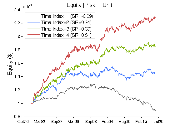
Figure 4 | Equity Curves for Scenario #2 (Table 3).
IV. Basic Concepts
B. Mandelbrot, The (mis)Behavior of Markets:
Trouble runs in streaks:
Market turbulence tends to cluster. This is no surprise to an experienced trader. In financial dealing-rooms across the world, the first fifteen minutes of trading each morning are critically important; it is when experienced traders, staring at their screens, take the temperature of the market. They know that when a market opens choppily, it may well continue that way. They know that a wild Tuesday may well be followed by a wilder Wednesday. And they also know that it is in those wildest moments – the rare but recurring crises of the financial world – that the biggest fortunes of Wall Street are made and lost. They need no economists to tell them all this. But their intuition, not included in the standard model of efficient markets, is entirely validated by the multifractal model.
V. Summary
Opening Range Breakout (ORB) does not improve the original volatility clustering model.
Related Entries: Volatility Clustering: Part 1 | Volatility Clustering: Part 2 | Narrow Range N-Day Pattern
Related Topics: (Public) Trading Strategies
CFTC RULE 4.41: HYPOTHETICAL OR SIMULATED PERFORMANCE RESULTS HAVE CERTAIN LIMITATIONS. UNLIKE AN ACTUAL PERFORMANCE RECORD, SIMULATED RESULTS DO NOT REPRESENT ACTUAL TRADING. ALSO, SINCE THE TRADES HAVE NOT BEEN EXECUTED, THE RESULTS MAY HAVE UNDER-OR-OVER COMPENSATED FOR THE IMPACT, IF ANY, OF CERTAIN MARKET FACTORS, SUCH AS LACK OF LIQUIDITY. SIMULATED TRADING PROGRAMS IN GENERAL ARE ALSO SUBJECT TO THE FACT THAT THEY ARE DESIGNED WITH THE BENEFIT OF HINDSIGHT. NO REPRESENTATION IS BEING MADE THAT ANY ACCOUNT WILL OR IS LIKELY TO ACHIEVE PROFIT OR LOSSES SIMILAR TO THOSE SHOWN.
RISK DISCLOSURE: U.S. GOVERNMENT REQUIRED DISCLAIMER | CFTC RULE 4.41
Codes: matlab/data/volatility-clustering-3