Greatest Swing Value – Trend | Trading Strategy (Filter & Exit)

I. Trading Strategy

Developer: Larry Williams. Concept: Volatility expansion with a trend bias. Research Goal: A benchmark test: Greatest Swing Value (GSV) – Trend vs. Opening Range Breakout (ORB). Specification: Table 1. Results: Figure 1-2. Trade Setup: N/A. Trade Entry: Greatest Swing Value (GSV). A trade is taken at a predetermined amount above/below the open. The predetermined amount is called the GSV. Long Trades: In a bullish mode, a buy stop is placed at [Open + GSV]. Short Trades: In a bearish mode, a sell stop is placed at [Open − GSV]. Trade Exit: Table 1. Portfolio: 42 futures markets from four major market sectors (commodities, currencies, interest rates, and equity indexes). Data: 32 years since 1980. Testing Platform: MATLAB®.

II. Sensitivity Test

All 3-D charts are followed by 2-D contour charts for Profit Factor, Sharpe Ratio, Ulcer Performance Index, CAGR, Maximum Drawdown, Percent Profitable Trades, and Avg. Win / Avg. Loss Ratio. The final picture shows sensitivity of Equity Curve.

Tested Variables: Trend_Index & Time_Index (Definitions: Table 1):

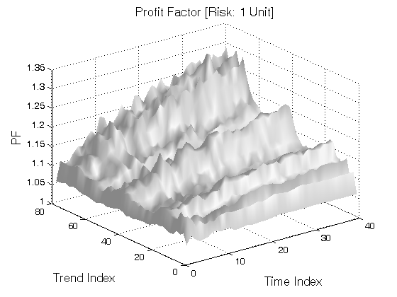
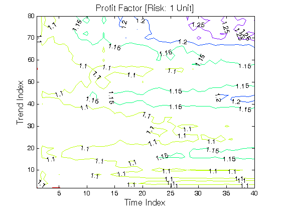
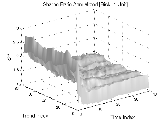
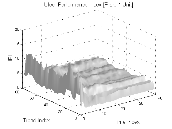
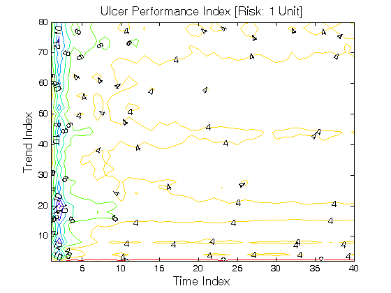
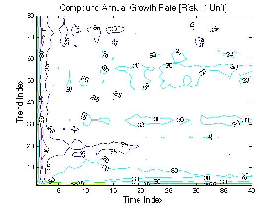
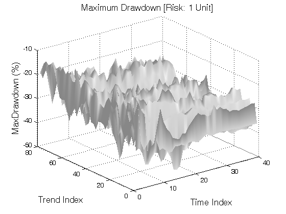
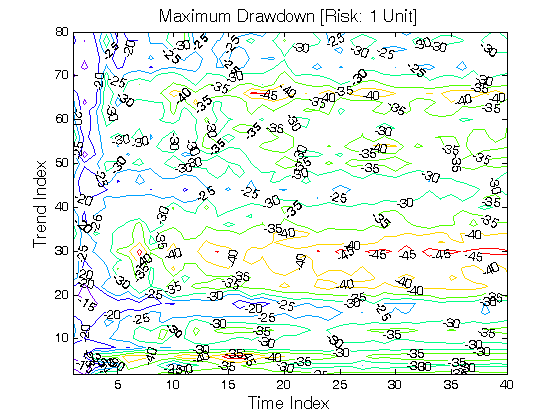
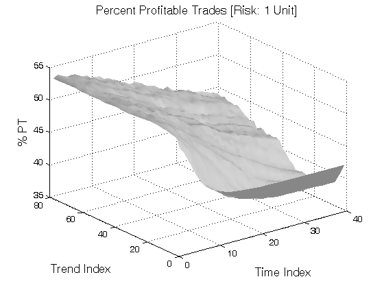
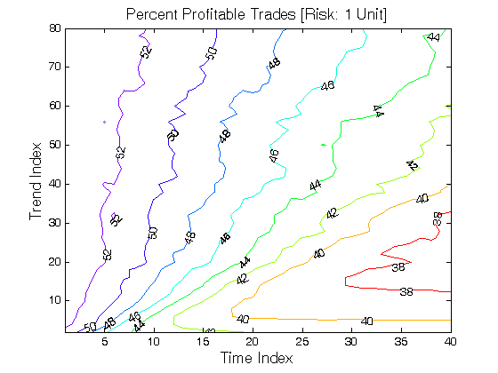
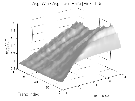
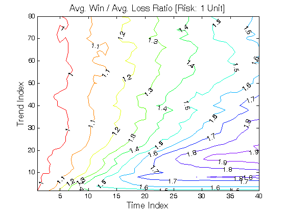
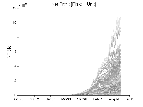
Figure 1 | Portfolio Performance (Inputs: Table 1; Commission & Slippage: $0).

STRATEGY	SPECIFICATION	PARAMETERS
Auxiliary Variables:	Noise: If Close[i] > Open[i] then Noise = Open[i] − Low[i]; If Close[i] < Open[i] then Noise = High[i] − Open[i]; If Close[i] = Open[i] then Noise = min(Open[i] − Low[i], High[i] − Open[i]). Index: i ~ Current Bar. Average_Noise: The simple moving average of Noise over a period of GSV_Length. GSV[i] = Average_Noise[i] * GSV_Multiple.	GSV_Length = 10; GSV_Multiple = 2;
Setup:	N/A
Filter:	Long Trades: Close[i − 1] > Close[i − Trend_Index]. Short Trades: Close[i − 1] < Close[i − Trend_Index]. Index: i ~ Current Bar.	Trend_Index = [2, 80], Step = 2;
Entry:	Greatest Swing Value (GSV). A trade is taken at a predetermined amount above/below the open. The predetermined amount is called the GSV (defined above). Long Trades: In a bullish mode, a buy stop is placed at [Open + GSV]. Short Trades: In a bearish mode, a sell stop is placed at [Open − GSV].
Exit:	Time Exit: nth day at the close, n = Time_Index. Stop Loss Exit: ATR(ATR_Length) is the Average True Range over a period of ATR_Length. ATR_Stop is a multiple of ATR(ATR_Length). Long Trades: A sell stop is placed at [Entry − ATR(ATR_Length) * ATR_Stop]. Short Trades: A buy stop is placed at [Entry + ATR(ATR_Length) * ATR_Stop].	Time_Index = [1, 40], Step = 1; ATR_Length = 20; ATR_Stop = 6;
Sensitivity Test:	Trend_Index = [2, 80], Step = 2 Time_Index = [1, 40], Step = 1
Position Sizing:	Initial_Capital = $1,000,000 Fixed_Fractional = 1% Portfolio = 42 US Futures ATR_Stop = 6 (ATR ~ Average True Range) ATR_Length = 20
Data:	42 futures markets; 32 years (1980/01/01−2011/12/31)

Table 1 | Specification: Trading Strategy.

III. Sensitivity Test with Commission & Slippage

Tested Variables: Trend_Index & Time_Index (Definitions: Table 1):

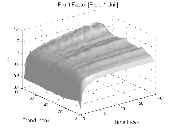
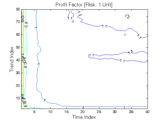
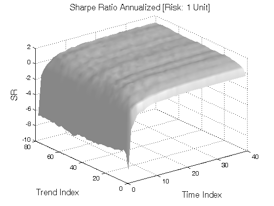
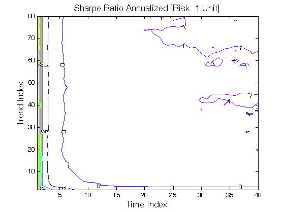
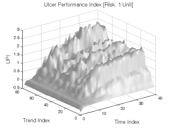
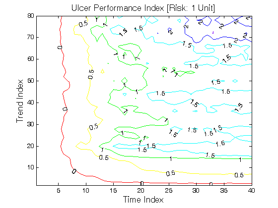
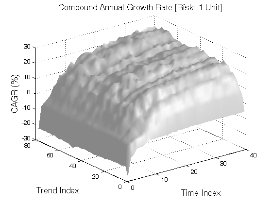
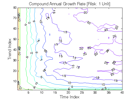
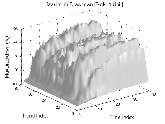
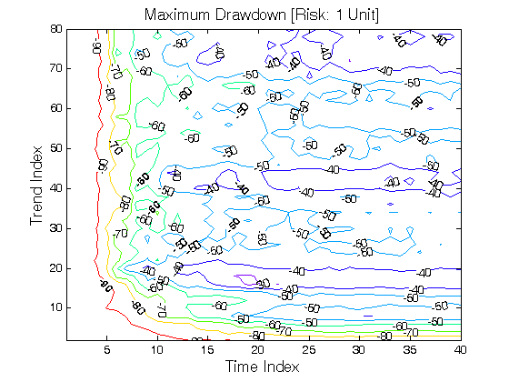
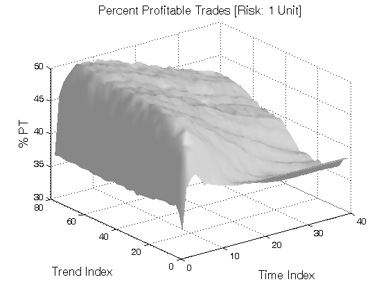
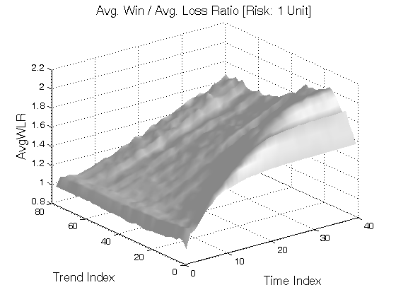
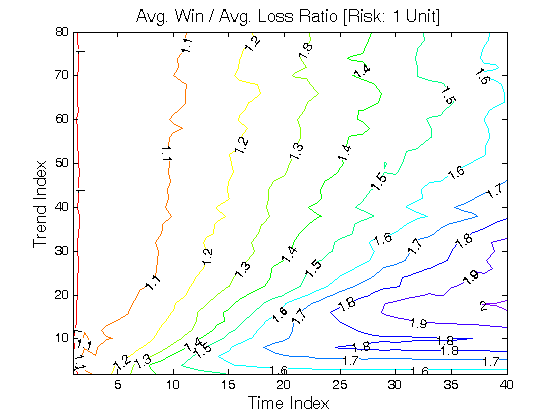
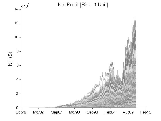
Figure 2 | Portfolio Performance (Inputs: Table 1; Commission & Slippage: $50 Round Turn).

IV. Rating: Greatest Swing Value – Trend | Trading Strategy

A/B/C/D

Related Entries: Greatest Swing Value (Exits) | Opening Range Breakout (Exits) | ORBP Trend (Filter & Exit) | ORBP Counter-Trend (Filter & Exit)
Related Topics: (Public) Trading Strategies

CFTC RULE 4.41: HYPOTHETICAL OR SIMULATED PERFORMANCE RESULTS HAVE CERTAIN LIMITATIONS. UNLIKE AN ACTUAL PERFORMANCE RECORD, SIMULATED RESULTS DO NOT REPRESENT ACTUAL TRADING. ALSO, SINCE THE TRADES HAVE NOT BEEN EXECUTED, THE RESULTS MAY HAVE UNDER-OR-OVER COMPENSATED FOR THE IMPACT, IF ANY, OF CERTAIN MARKET FACTORS, SUCH AS LACK OF LIQUIDITY. SIMULATED TRADING PROGRAMS IN GENERAL ARE ALSO SUBJECT TO THE FACT THAT THEY ARE DESIGNED WITH THE BENEFIT OF HINDSIGHT. NO REPRESENTATION IS BEING MADE THAT ANY ACCOUNT WILL OR IS LIKELY TO ACHIEVE PROFIT OR LOSSES SIMILAR TO THOSE SHOWN.

RISK DISCLOSURE: U.S. GOVERNMENT REQUIRED DISCLAIMER | CFTC RULE 4.41

Codes: matlab/williams/gsv/a/tf